< B.6 Homework 6 | Contents | B.8 Homework 8 >
![]()
This notebook contains material from chemeng316_fluids; content is available on Github.
< B.6 Homework 6 | Contents | B.8 Homework 8 >
![]()
Getting Started: See prior homework templates fFor sample code to import the pint, CoolProp, numpy, sympy, and matplotlib modules.
Problem 1. A liquid is flowing steadily through a 75 mm pipe. The local velocity varies with distance from the pipe axis as shown in the table below. Calculate (a) the average velocity $\overline{V}$, (b) the kinetic-energy correction factor, $\alpha$, and (c) the momentum correction factor, $\beta$. YES, this problem does say the flow is in a PIPE, so you have to integrate the velocity over the cylindrical area of the pipe. The area for a single $dA$ ring is $dA = 2\pi\,r\,dr$. Remember, integration is just summing up area, so the numerical integration for the average velocity looks like this:
$$ \overline{V} = \sum_{i-1}^{N}u_i\, 2\pi\,r_i\,\Delta_r $$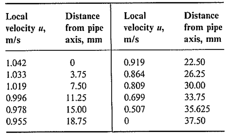
# YOUR SOLUTION HERE
Problem 2. A water tank is 30 feet in diameter and is filled to a depth of 25 feet. The outlet is a 4 inch diameter opening. (a) What is the initial volumetric flow rate from the tank? (b) How long will it take for the tank to be empty? (c) Calculate the average flow rate (you have to integrate using results from part (b)) and compare it to the initial flow rate.
# YOUR SOLUTION HERE
< B.6 Homework 6 | Contents | B.8 Homework 8 >
![]()